Importance of RLS
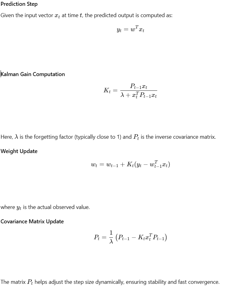
Recursive Least Squares (RLS) is an adaptive filtering algorithm widely used for real-time signal processing, system identification, and time-series prediction. Unlike standard least squares, RLS dynamically updates model parameters as new data arrives, making it well-suited for non-stationary environments.
RLS Use Cases
RLS has numerous real-world applications, such as:
- Financial Forecasting: Predicting stock prices based on historical data.
- Control Systems: Adapting controller parameters in real-time for dynamic systems.
- IoT and Sensor Networks: Filtering and predicting sensor data to reduce noise and improve reliability.
- Speech Processing: Noise cancellation and adaptive equalization.
Technical Details of RLS
RLS operates by minimizing the weighted least squares error iteratively. The algorithm maintains an estimate of the weight vector ww, which updates with each new observation. The core equations of RLS include:
Implementation in Python
Below is an implementation of RLS for time-series prediction, integrated with an internal timer to periodically reset the model and improve stability:
import numpy as np

# Initialize global variables for RLS-based time-series prediction
reset_interval_steps = 100  # Interval to reset the model (500 steps = 5 seconds with 0.01s step time)
sequence_length = sequence_length = int(reset_interval_steps / 10)  # Sequence length to retain more historical data
input_sequence = []  # Stores the past sensor values for prediction
P = np.eye(sequence_length) * 1000  # Covariance matrix
w = np.zeros((sequence_length, 1))  # Weight vector
lambda_factor = 0.95  # Forgetting factor for better stability
actual_values = []  # To track real sensor data
predicted_values = []  # To track predicted values
step_counter = 0  # Step counter to track time steps


def python_init():
    global input_sequence, P, w, actual_values, predicted_values, step_counter
    input_sequence = []
    P = np.eye(sequence_length) * 1000
    w = np.zeros((sequence_length, 1))
    actual_values = []
    predicted_values = []
    step_counter = 0  # Reset step counter
    print("RLS-based time series prediction system initialized.")

def python_inout(inputs):
    """
    Predict the value at steps_ahead and evaluate MSE and R².
    Args:
        inputs (numpy array): Array where inputs[0] is the sensor value and inputs[1] is steps_ahead.
    Returns:
        numpy array: Predicted value, MSE, and R².
    """
    global input_sequence, P, w, lambda_factor, actual_values, predicted_values, step_counter

    # Increment the step counter
    step_counter += 1

    # Check if the step counter has reached the reset interval and reset if needed
    if step_counter >= reset_interval_steps:
        # Reset model state every reset_interval_steps
        python_init()

    sensor_value = inputs[0]  # Sensor value at the current time step
    steps_ahead = int(inputs[1])  # Steps ahead to predict

    # Update the sequence with the new sensor value
    input_sequence.append(sensor_value)
    actual_values.append(sensor_value)  # Store the actual sensor reading

    # Maintain the fixed sequence length
    if len(input_sequence) > sequence_length:
        input_sequence.pop(0)

    # Predict only if enough data exists
    if len(input_sequence) < sequence_length:
        return np.array([0.0] * steps_ahead + [np.nan] * 2)  # Not enough data for prediction

    # Prepare the input vector for RLS
    x = np.array(input_sequence).reshape(sequence_length, 1)

    # Make predictions for the next 'steps_ahead' values
    future_prediction = None
    last_predicted_value = sensor_value  # Start with the real sensor value

    for i in range(steps_ahead):
        # Use real values until the last step (freezing the first part of the predictions)
        if i == 0:
            predicted_value = float(np.dot(w.T, x))  # Predict the next value based on current input
        else:
            predicted_value = float(np.dot(w.T, x))  # Continue using predictions from previous steps

        # Store the prediction at the required step (steps_ahead-th)
        if i == steps_ahead - 1:
            future_prediction = predicted_value

        # Perform the RLS update with real sensor data
        x_T = x.T
        K = P @ x / (lambda_factor + x_T @ P @ x)  # Kalman gain
        w = w + K * (sensor_value - float(x_T @ w))  # Update weights
        P = (P - K @ x_T @ P) / lambda_factor  # Update covariance matrix

        # Apply a small regularization term to the covariance matrix to prevent instability
        P += 1e-6 * np.eye(sequence_length)

        # Update x with the predicted value for the next iteration
        x = np.roll(x, -1, axis=0)
        x[-1] = predicted_value

    predicted_values.append(future_prediction)  # Store the prediction

    # Calculate MSE and R² over the last 10 values (warm-up period + prediction)
    if len(actual_values) >= 10 and len(predicted_values) >= 10:
        mse = np.mean((np.array(actual_values[-10:]) - np.array(predicted_values[-10:])) ** 2)  # MSE
        ss_total = np.sum((np.array(actual_values[-10:]) - np.mean(actual_values[-10:])) ** 2)  # Total sum of squares
        ss_residual = np.sum((np.array(actual_values[-10:]) - np.array(predicted_values[-10:])) ** 2)  # Residual sum of squares
        r2 = 1 - (ss_residual / ss_total)  # R²

        return np.array([future_prediction, mse, r2])

    return np.array([future_prediction, np.nan, np.nan])

def python_end():
    """
    Finalize the prediction block.
    """
    print("RLS-based time series prediction block finished executing.")
Here is a video demo
How Twin Simulate Facilitates RLS-Based Development
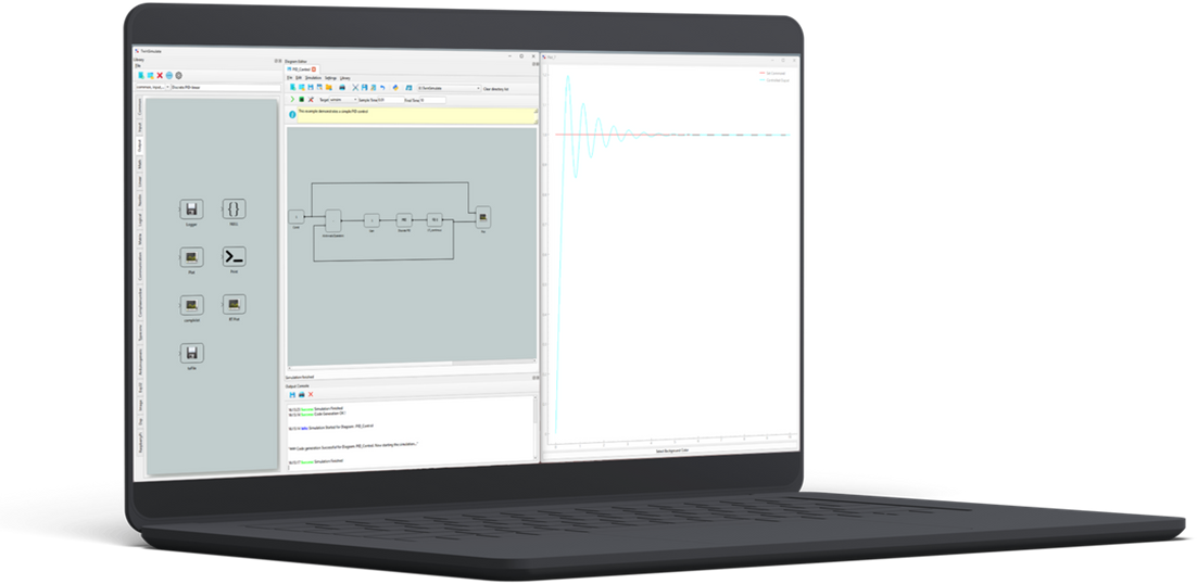
TwinSimulate provides a model-based approach to implementing and testing RLS algorithms in a realistic environment. With TwinSimulate, users can:
- Integrate RLS with IoT and MQTT-based data streams for real-time prediction and decision-making.
- Simulate sensor-driven environments to test adaptive algorithms before deployment.
- Leverage pre-built blocks to implement and refine predictive models without extensive manual coding.
By combining RLS with digital twin technology, TwinSimulate enables rapid prototyping and deployment of adaptive filtering solutions across multiple domains. Whether for industrial automation, predictive maintenance, or real-time analytics, TwinSimulate ensures seamless integration and validation of RLS models in practical applications.
Road map for easy to use blocks in Twin Simulate
Let us know if this looks a good list or we do something else ?
Kalman Filter – A recursive Bayesian filter widely used for tracking and prediction in dynamic systems.
Extended Kalman Filter (EKF) – A nonlinear extension of the Kalman filter that linearizes the system dynamics.
Unscented Kalman Filter (UKF) – An improved nonlinear Kalman filter using sigma points instead of linearization.
Particle Filter – A Monte Carlo-based Bayesian filtering method for non-Gaussian and nonlinear systems.
Least Mean Squares (LMS) – A simple adaptive filtering algorithm used for noise cancellation and equalization.
Normalized Least Mean Squares (NLMS) – An improvement over LMS with normalized step size for faster convergence.
Conjugate Gradient (CG) Algorithm – A method for solving large-scale least-squares problems efficiently.
Expectation-Maximization (EM) Algorithm – A probabilistic method used in Gaussian Mixture Models (GMM) and hidden Markov models (HMM).
Support Vector Regression (SVR) – A machine learning approach for regression and time-series prediction.
Autoregressive Integrated Moving Average (ARIMA) – A statistical method widely used in time-series forecasting.
Long Short-Term Memory (LSTM) Networks – A type of recurrent neural network (RNN) specialized for sequential data.
Gated Recurrent Units (GRU) – A simplified version of LSTM with fewer parameters.
Fourier Transform-Based Filtering – Used for frequency-domain analysis and filtering in time-series data.
Wavelet Transform-Based Filtering – A multi-resolution analysis technique useful for non-stationary signals.
Adaptive Neuro-Fuzzy Inference System (ANFIS) – A hybrid of neural networks and fuzzy logic for adaptive modeling.


